Intermediate Tutorial - Prepare Data & Multi-Algorithm Runs

This tutorial builds on the introduction to SPRAS from the previous tutorial.

It guides participants through how to convert data into a format usable by pathway reconstruction algorithms, run multiple algorithms within a single workflow, and apply new tools to interpret and compare the resulting pathways.

You will learn how to:

• Prepare and format data for use with SPRAS

• Configure and run additional pathway reconstruction algorithms on a dataset

• Enable post-analysis steps to generate post analysis information

Step 1: Transforming high throughput experimental data into SPRAS compatible input data

1.1 What is the SPRAS-standardized input data?

A pathway reconstruction algorithm requires a set of input nodes and an interactome; however, each algorithm expects its inputs to follow a unique format.

To simplify this process, SPRAS requires all input data in a dataset to be formatted once into a standardized SPRAS format. SPRAS then automatically generates algorithm-specific input files when an algorithm is enabled in the configuration file.

Note

Each algorithm uses the input nodes to guide or constrain the optimization process used to construct reconstruct subnetworks.

An algorithm maps these input nodes onto the interactome and uses the network to identify connecting paths between the input nodes to form subnetworks.

Pathway reconstruction algorithms differ in the inputs nodes they require and how they interpret those nodes to identify subnetworks.

• Some use source and target nodes to defined start and end points.

• Some use prizes, which assign numerical scores assigned to nodes of interest.

• Some rely on active nodes, representing nodes that are significantly “on” under specific conditions.

An example of a node file required by SPRAS follows a tab-separated format:

NODEID  prize sources targets active
A       1.0     True            True
B       3.3             True    True
C       2.5     True            True
D       1.9             True    True

Note

If a user provides only one type of input node but wants to run algorithms that require a different type, SPRAS can automatically convert the inputs into the compatible format:

• Source-target nodes can be used with all algorithms by making a prize column set to 1 and an active column set to True.

• Prize data can be adapted for active based algorithms by automatically making an active column set to True.

• Active data can be adapted for prize based algorithms by making a prize column set to 1.

Along with differences in their inputs nodes, pathway reconstruction algorithms also interpret the input interactome differently.

• Some algorithms can handle only fully directed interactomes. These interactomes include edges with a specific direction (A -> B).

• Others work only with fully undirected interactomes. These interactomes have edges without direction (A - B).

• And some support mixed-directionaltiy interactomes. These interactomes contain both directed and undirected edges.

SPRAS automatically converts the user-provided edge file into the format expected by each algorithm, ensuring that the directionality of the interactome matches the algorithm’s requirements.

An example of an edge file required by SPRAS follows a tab-separated format. where U indicates an undirected edge and D indicates a directed edge:

A   B   0.98   U
B   C   0.77   D

Note

SPRAS supports multiple standardized input formats. More information about input data formats can be found in the inputs/README.md file within the SPRAS repository.

1.2 Example high throughput data

An example dataset is using EGF response mass spectrometry data [4]. The experiment for this data was repeated three times, known as biological replicates, to ensure the results are consistent. Each replicate measures the abundance of peptides at different time points (0-128 minutes) to capture how protein activity changes over time.

Note

Mass spectrometry is a technique used to measure and identify proteins in a sample. It works by breaking proteins into smaller pieces called peptides and measuring their mass-to-charge ratio, which enables identifying which peptide is being measured. The data show how much of each peptide is present, which can show how protein phosphorylation abundances change under different conditions.

Since proteins interact with each other in biological pathways, changes in their phosphorylation abundances can reveal which parts of a pathway are active or affected. By mapping these changing proteins onto known interaction networks, pathway reconstruction algorithms can identify which signaling pathways are likely involved in the biological response to a specific condition.

Example of one of the biological replicate A with one peptide:

peptide	protein	gene.name	modified.sites	0 min	2 min	4 min	8 min	16 min	32 min	64 min	128 mn
K.n[305.21]AFWMAIGGDRDEIEGLS[167.00]S[167.00]DEEH.-	Q6PD74,B4DG44,Q5JPJ4,Q6AWA0	AAGAB	S310,S311	14.97	14.81	13.99	13.98	12.87	13.88	13.91	15.60

The goal is to turn this experimental data into the format that SPRAS expects.

1.3 Filtering and normalizing the replicates

Before analysis, we filter out peptides not present in all three replicates to ensure consistency. Then, we normalize each replicate so intensity values are comparable and not biased by replicate-specific effects.

peptide	protein	gene.name	modified.sites	0 min	2 min	4 min	8 min	16 min	32 min	64 min	128 mn	replicate
K.n[305.21]AFWMAIGGDRDEIEGLS[167.00]S[167.00]DEEH.-	Q6PD74,B4DG44,Q5JPJ4,Q6AWA0	AAGAB	S310,S311	2.17	2.09	1.98	1.78	1.99	2.12	2.25	1.46	C
K.n[305.21]AFWMAIGGDRDEIEGLS[167.00]S[167.00]DEEH.-	Q6PD74,B4DG44,Q5JPJ4,Q6AWA0	AAGAB	S310,S311	4.03	3.73	3.32	3.36	3.35	3.37	3.35	3.86	B
K.n[305.21]AFWMAIGGDRDEIEGLS[167.00]S[167.00]DEEH.-	Q6PD74,B4DG44,Q5JPJ4,Q6AWA0	AAGAB	S310,S311	5.60	4.75	4.69	4.59	4.32	4.90	4.90	5.48	A

1.4 Computing p-values using Tukey’s HSD Test

We want to calculate the p-values per peptide. This tells us how likely changes in abundance happen by chance.

We use Tukey’s Honest Significant Difference (HSD) test to compare all time points and correct for multiple testing to get a p-value for every pair of time points.

peptide	protein	2min vs 0min	4min vs 0min	8min vs 0min	16min vs 0min	32min.vs.0min	64min.vs.0min	128min.vs.0min	4min.vs.2min	8min.vs.2min	16min.vs.2min	32min.vs.2min	64min.vs.2min	128min.vs.2min	8min.vs.4min	16min.vs.4min	32min.vs.4min	64min.vs.4min	128min.vs.4min	16min.vs.8min	32min.vs.8min	64min.vs.8min	128min.vs.8min	32min.vs.16min	64min.vs.16min	128min.vs.16min	64min.vs.32min	128min.vs.32min	128min.vs.64min
K.n[305.21]ADVLEAHEAEAEEPEAGK[432.30]S[167.00]EAEDDEDEVDDLPSSR.R	QQ6PD74,B4DG44,Q5JPJ4,Q6AWA0	0.67	0.25	0.14	0.12	0.52	0.76	0.84	0.99	0.93	0.90	1.00	1.00	1.00	1.00	1.00	1.00	0.97	0.94	1.00	0.98	0.87	0.80	0.96	0.83	0.75	1.00	1.00	1.00

Peptides with lower p-values are more statistically significant and may represent biologically meaningful changes in phosphorylation over time.

1.5 From p-values to prizes

P-values are transformed using -log10(p-value) so smaller p-values give larger prize scores.

For each peptide, the smallest p-value is selected (representing the most significant change) between each time point to the baseline (0 min) and between consecutive time points. This is because the ultimate network analysis will not use the temporal information.

For each protein mapped to multiple peptides, the maximum prize value across all its peptides is assigned.

Finally, all protein identifiers (using the first one listed for each protein) are converted to UniProt Entry Names to match the identifiers that will be used in the interactome.

Note

All node identifiers should use the same namespace across every part of the data in a dataset.

peptide	protein	uniprot entry name	min p-value	-log10(min p-value)
K.n[305.21]AFWMAIGGDRDEIEGLS[167.00]S[167.00]DEEH.-	Q6PD74,B4DG44,Q5JPJ4,Q6AWA0	AAGAB_HUMAN	0.12392034609392	0.906857382317364

Input node data put into a SPRAS-standardized format:

NODE_ID     prize
AAGAB_HUMAN 0.906857382

1.6 From Prizes to Source and Targets / Actives

Using known pathway knowledge [1] [2] [3]:

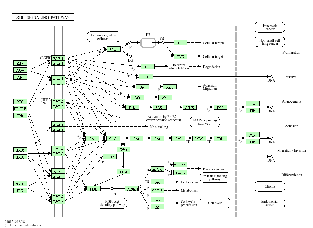
• EGF serves as a source for the pathway and was the experimental treatment.

• EGF is known to initiate signaling, so it can be added and assigned a high score (greater than all other nodes) to emphasize its importance and guide algorithms to start reconstruction from this point. (EGF is currently not in the data)

• EGFR is in the current data. Looking at the pathway, we can see that EGFR directly interacts with EGF in the pathway.

• All other downstream proteins detected in the data can also treated as targets.

• All proteins in the data can be considered active since they correspond to proteins that are active under the given biological condition.

Input node data put into a SPRAS-standardized format:

NODE_ID     prize       source  target  active
AAGAB_HUMAN 0.906857382         True   True
... more nodes
EGF_HUMAN   10              True    True    True
EGFR_HUMAN  6.787874699                 True        True
... more nodes

1.8 Finding an Interactome to use

To connect our proteins, we use a background protein-protein interaction (PPI) network (the interactome). For this dataset, two interactomes are merged (directed edges prioritized when available):

• iRefIndex v13 (159,095 undirected interactions)

• PhosphoSitePlus (4,080 directed kinase-substrate interactions)

The final network has 15,677 proteins and 157,984 edges (~4k of them are directed), and covers 653 of our 702 prize proteins. The proteins identifiers in the interactome are converted to use UniProt Entry Names.

Interactome data put into a SPRAS-standardized format:

TACC1_HUMAN RUXG_HUMAN      0.736771        U
TACC1_HUMAN KAT2A_HUMAN     0.292198        U
TACC1_HUMAN CKAP5_HUMAN     0.724783        U
TACC1_HUMAN YETS4_HUMAN     0.542597        U
TACC1_HUMAN LSM7_HUMAN      0.714823        U
AURKC_HUMAN TACC1_HUMAN     0.553333        D
TACC1_HUMAN AURKA_HUMAN     0.401165        U
TACC1_HUMAN KDM1A_HUMAN     0.367850        U
TACC1_HUMAN MEMO1_HUMAN     0.367850        U
TACC1_HUMAN HD_HUMAN        0.367850        U
... more edges

Note

Many databases exist that provide interactomes. One is STRING, which contains known protein-protein interactions across different species.

1.9 This SPRAS-standardized data is already saved into SPRAS

spras/
├── .snakemake/
│   └── log/
│       └── ... snakemake log files ...
├── config/
│   └── ...
├── inputs/
│   ├── phosphosite-irefindex13.0-uniprot.txt # pre-defined in SPRAS already, used by the intermediate.yaml file
│   └── tps-egfr-prizes.txt # pre-defined in SPRAS already, used by the intermediate.yaml file
├── outputs/
│   └── basic/
│       └── ... output files ...

The data used in this part of the tutorial can be found in the supplementary materials under data supplement 2 and supplement 3 [4].

Step 2: Running multiple algorithms

We can begin running multiple pathway reconstruction algorithms.

For this part of the tutorial, we’ll use a pre-defined configuration file that includes additional algorithms and post-analysis steps available in SPRAS. Download it here: Intermediate Config File

Save the file into the config/ folder of your SPRAS installation.

After adding this file, your directory structure will look like this (ignoring the rest of the folders):

spras/
├── .snakemake/
│   └── log/
│       └── ... snakemake log files ...
├── config/
│   ├── basic.yaml
│   ├── intermediate.yaml
│   └── ... other configs ...
├── inputs/
│   ├── phosphosite-irefindex13.0-uniprot.txt # pre-defined in SPRAS already, used by the intermediate.yaml file
│   ├── tps-egfr-prizes.txt # pre-defined in SPRAS already, used by the intermediate.yaml file
│   └── ... other input data ...
├── outputs/
│   └── basic/
│       └── ... output files ...

2.1 Algorithms in SPRAS

SPRAS supports a wide range of algorithms, each designed around different biological assumptions and optimization strategies (See Pathway Reconstruction Methods for SPRAS’s list of integrated algorithms.)

Wrapped algorithms

Each pathway reconstruction algorithm within SPRAS has been wrapped for SPRAS, meaning it has been prepared for the SPRAS framework.

For an algorithm-specific wrapper, the wrapper includes a module that will create and format the input files required by the algorithm using the SPRAS-standardized input data.

Each algorithm has an associated Docker image located on DockerHub that contains all necessary software dependencies needed to run it. For an algorithm-specific wrapper, it contains a module that will call each image to launch a container for a specified parameter combination, set of prepared algorithm-specific inputs and an output filename (raw-pathway.txt).

With each of the raw-pathway.txt files, an algorithm-specific wrapper includes a module that will convert the algorithm-specific format into a standardized SPRAS format.

2.3 Running SPRAS with multiple algorithms

In the intermediate.yaml configuration file, it is set up to have SPRAS run multiple algorithms with multiple parameter settings on a single dataset.

From the root directory, run the command below from the command line:

snakemake --cores 4 --configfile config/intermediate.yaml

What happens when you run this command

SPRAS will run “slower” when using the intermediate.yaml configuration.

Similar automated steps from the previous tutorial runs behind the scenes for intermediate.yaml. However, this configuration now runs multiple algorithms with different parameter combinations, which takes longer to complete. By increasing the number of cores to 4, it allows Snakemake to parallelize the work locally, speeding up execution when possible. (See Using SPRAS for more information on SPRAS’s parallelization.)

1. Snakemake starts the workflow

Snakemake reads the options set in the intermediate.yaml configuration file and determines which datasets, algorithms, and parameter combinations need to run. It also checks if any post-analysis steps were requested.

2. Creating algorithm-specific inputs

For each algorithm marked as include: true in the configuration, SPRAS generates input files tailored to that algorithm.

In this case, every algorithm is enabled, so SPRAS formats the input files required for each algorithm.

3. Organizing results with parameter hashes

Each <dataset>-<algorithm>-params-<hash> combination gets its own folder created in output/intermediate/.

A matching log file in logs/parameters-<algorithm>-params-<hash>.yaml records the exact parameter values used.

4. Running the algorithm

SPRAS pulls each algorithm’s Docker image from DockerHub if it isn’t already downloaded locally

SPRAS executes each algorithm by launching multiple Docker contatiners using the algorithm-specific Docker image (once for each parameter configuration), sending the prepared input files and specific parameter settings needed for execution.

Each algorithm runs independently within its Docker container and generates an output file named raw-pathway.txt, which contains the reconstructed subnetwork in the algorithm-specific format.

SPRAS then saves these files to the corresponding folder.

5. Standardizing the results

SPRAS parses each of the raw output into a standardized SPRAS format (pathway.txt) and SPRAS saves this file in its corresponding folder.

6. Logging the Snakemake run

Snakemake creates a dated log in .snakemake/log/ This log shows what jobs ran and any errors that occurred during the SPRAS run.

What your directory structure should like after this run:

spras/
├── .snakemake/
│   └── log/
│       └── ... snakemake log files ...
├── config/
│   └── basic.yaml
├── inputs/
│   ├── phosphosite-irefindex13.0-uniprot.txt
│   └── tps-egfr-prizes.txt
├── outputs/
│   └── basic/
│       └── dataset-egfr-merged.pickle
│       └── egfr-meo-params-FJBHHNE
│            └── pathway.txt
│            └── raw-pathway.txt
│       └── egfr-meo-params-GKEDDFZ
│            └── pathway.txt
│            └── raw-pathway.txt
│       └── egfr-meo-params-JQ4DL7K
│            └── pathway.txt
│            └── raw-pathway.txt
│       └── egfr-meo-params-OXXIFMZ
│            └── pathway.txt
│            └── raw-pathway.txt
│       └── egfr-mincostflow-params-42UBTQI
│            └── pathway.txt
│            └── raw-pathway.txt
│       └── egfr-mincostflow-params-4G2PQRB
│            └── pathway.txt
│            └── raw-pathway.txt
│       └── egfr-omicsintegrator1-params-FZI2OGW
│            └── pathway.txt
│            └── raw-pathway.txt
│       └── egfr-omicsintegrator1-params-GUMLBDZ
│            └── pathway.txt
│            └── raw-pathway.txt
│       └── egfr-omicsintegrator1-params-PCWFPQW
│            └── pathway.txt
│            └── raw-pathway.txt
│       └── egfr-omicsintegrator2-params-EHHWPMD
│            └── pathway.txt
│            └── raw-pathway.txt
│       └── egfr-omicsintegrator2-params-IV3IPCJ
│            └── pathway.txt
│            └── raw-pathway.txt
│       └── egfr-pathlinker-params-4YXABT7
│            └── pathway.txt
│            └── raw-pathway.txt
│       └── egfr-pathlinker-params-7S4SLU6
│            └── pathway.txt
│            └── raw-pathway.txt
│       └── egfr-pathlinker-params-D4TUKMX
│            └── pathway.txt
│            └── raw-pathway.txt
│       └── egfr-pathlinker-params-VQL7BDZ
│            └── pathway.txt
│            └── raw-pathway.txt
│       └── egfr-rwr-params-34NN6EK
│            └── pathway.txt
│            └── raw-pathway.txt
│       └── egfr-rwr-params-GGZCZBU
│            └── pathway.txt
│            └── raw-pathway.txt
│       └── egfr-strwr-params-34NN6EK
│            └── pathway.txt
│            └── raw-pathway.txt
│       └── egfr-strwr-params-GGZCZBU
│            └── pathway.txt
│            └── raw-pathway.txt
│       └── logs
│            └── datasets-egfr.yaml
│            └── parameters-allpairs-params-BEH6YB2.yaml
│            └── parameters-domino-params-V3X4RW7.yaml
│            └── parameters-meo-params-FJBHHNE.yaml
│            └── parameters-meo-params-GKEDDFZ.yaml
│            └── parameters-meo-params-JQ4DL7K.yaml
│            └── parameters-meo-params-OXXIFMZ.yaml
│            └── parameters-mincostflow-params-42UBTQI.yaml
│            └── parameters-mincostflow-params-4G2PQRB.yaml
│            └── parameters-mincostflow-params-GGT4CVE.yaml
│            └── parameters-omicsintegrator1-params-FZI2OGW.yaml
│            └── parameters-omicsintegrator1-params-GUMLBDZ.yaml
│            └── parameters-omicsintegrator1-params-PCWFPQW.yaml
│            └── parameters-omicsintegrator2-params-EHHWPMD.yaml
│            └── parameters-omicsintegrator2-params-IV3IPCJ.yaml
│            └── parameters-pathlinker-params-4YXABT7.yaml
│            └── parameters-pathlinker-params-7S4SLU6.yaml
│            └── parameters-pathlinker-params-D4TUKMX.yaml
│            └── parameters-pathlinker-params-VQL7BDZ.yaml
│            └── parameters-rwr-params-34NN6EK.yaml
│            └── parameters-rwr-params-GGZCZBU.yaml
│            └── parameters-strwr-params-34NN6EK.yaml
│            └── parameters-strwr-params-GGZCZBU.yaml
│       └── prepared
│            └── egfr-domino-inputs
│                ├── active_genes.txt
│                └── network.txt
│            └── egfr-meo-inputs
│                ├── edges.txt
│                ├── sources.txt
│                └── targets.txt
│            └── egfr-mincostflow-inputs
│                ├── edges.txt
│                ├── sources.txt
│                └── targets.txt
│            └── egfr-omicsintegrator1-inputs
│                ├── dummy_nodes.txt
│                ├── edges.txt
│                └── prizes.txt
│            └── egfr-omicsintegrator2-inputs
│                ├── edges.txt
│                └── prizes.txt
│            └── egfr-pathlinker-inputs
│                ├── network.txt
│                ── nodetypes.txt
│            └── egfr-rwr-inputs
│                ├── network.txt
│                └── nodes.txt
│            └── egfr-strwr-inputs
|                ├── network.txt
|                ├── sources.txt
|                └── targets.txt

2.4 Reviewing the pathway.txt files

After running the intermediate configuration file, the output/intermediate/ directory will contain many more subfolders and files.

Again, each pathway.txt file contains the standardized reconstructed subnetworks and can be used at face value, or for further post analysis.

1. Locate the files

Navigate to the output directory output/intermediate/. Inside, you will find subfolders corresponding to each <dataset>-<algorithm>-params-<hash> combination.

2. Open a pathway.txt file

Each file lists the network edges that were reconstructed for that specific run. The format includes columns for the two interacting nodes, the rank, and the edge direction.

For example, the file egfr-mincostflow-params-42UBTQI/pathway.txt contains the following reconstructed subnetwork:

Node1       Node2   Rank    Direction
CBL_HUMAN   EGFR_HUMAN      1       U
EGFR_HUMAN  EGF_HUMAN       1       U
EMD_HUMAN   LMNA_HUMAN      1       U
FYN_HUMAN   KS6A3_HUMAN     1       U
EGF_HUMAN   HDAC6_HUMAN     1       U
HDAC6_HUMAN HS90A_HUMAN     1       U
KS6A3_HUMAN SRC_HUMAN       1       U
EGF_HUMAN   LMNA_HUMAN      1       U
MYH9_HUMAN  S10A4_HUMAN     1       U
EGF_HUMAN   S10A4_HUMAN     1       U
EMD_HUMAN   SRC_HUMAN       1       U

And the file egfr-omicsintegrator1-params-GUMLBDZ/pathway.txt contains the following reconstructed subnetwork:

Node1       Node2   Rank    Direction
CBLB_HUMAN  EGFR_HUMAN      1       U
CBL_HUMAN   CD2AP_HUMAN     1       U
CBL_HUMAN   CRKL_HUMAN      1       U
CBL_HUMAN   EGFR_HUMAN      1       U
CBL_HUMAN   PLCG1_HUMAN     1       U
CDK1_HUMAN  NPM_HUMAN       1       D
CHD4_HUMAN  HDAC2_HUMAN     1       U
EGFR_HUMAN  EGF_HUMAN       1       U
EGFR_HUMAN  GRB2_HUMAN      1       U
EIF3B_HUMAN EIF3G_HUMAN     1       U
FAK1_HUMAN  PAXI_HUMAN      1       U
GAB1_HUMAN  PTN11_HUMAN     1       U
GRB2_HUMAN  PTN11_HUMAN     1       U
GRB2_HUMAN  SHC1_HUMAN      1       U
HDAC2_HUMAN SIN3A_HUMAN     1       U
HGS_HUMAN   STAM2_HUMAN     1       U
KS6A1_HUMAN MK01_HUMAN      1       U
MK01_HUMAN  ABI1_HUMAN      1       D
MK01_HUMAN  ERF_HUMAN       1       D
MRE11_HUMAN RAD50_HUMAN     1       U

Step 3: Use ML post-analysis

3.1 Adding ML post-analysis to the intermediate configuration

To enable the ML analysis, update the analysis section in your configuration file by setting ml to true. Your analysis section in the configuration file should look like this:

analysis:
    ml:
        include: true
        ... (other parameters preset)

ml will perform unsupervised analyses such as principal component analysis (PCA), hierarchical agglomerative clustering (HAC), ensembling, and jaccard similarity comparisons of the pathways.

• The ml section includes configurable parameters that let you adjust the behavior of the analyses performed.

With these updates, SPRAS will run the full set of unsupervised machine learning analyses across all outputs for a given dataset.

After saving the changes in the configuration file, rerun with:

snakemake --cores 4 --configfile config/intermediate.yaml

What happens when you run this command

1. Reusing cached results

Snakemake reads the options set in intermediate.yaml and checks for any requested post-analysis steps. It reuses cached results; here the pathway.txt files generated from the previously executed algorithms on the egfr dataset are reused.

2. Running the ml analysis

SPRAS aggregates all the reconstructed subnetworks produced across the specified algorithms for a given dataset. SPRAS then performs machine learning analyses on each these groups and saves the results in the <dataset>-ml/ (egfr-ml/) folder.

What your directory structure should like after this run:

spras/
├── .snakemake/
│   └── log/
│       └── ... snakemake log files ...
├── config/
│   └── basic.yaml
├── inputs/
│   ├── phosphosite-irefindex13.0-uniprot.txt
│   └── tps-egfr-prizes.txt
├── outputs/
│   └── basic/
│       └── dataset-egfr-merged.pickle
│       └── egfr-meo-params-FJBHHNE
│            └── pathway.txt
│            └── raw-pathway.txt
│       └── egfr-meo-params-GKEDDFZ
│            └── pathway.txt
│            └── raw-pathway.txt
│       └── egfr-meo-params-JQ4DL7K
│            └── pathway.txt
│            └── raw-pathway.txt
│       └── egfr-meo-params-OXXIFMZ
│            └── pathway.txt
│            └── raw-pathway.txt
│       └── egfr-mincostflow-params-42UBTQI
│            └── pathway.txt
│            └── raw-pathway.txt
│       └── egfr-mincostflow-params-4G2PQRB
│            └── pathway.txt
│            └── raw-pathway.txt
│       └── egfr-omicsintegrator1-params-FZI2OGW
│            └── pathway.txt
│            └── raw-pathway.txt
│       └── egfr-omicsintegrator1-params-GUMLBDZ
│            └── pathway.txt
│            └── raw-pathway.txt
│       └── egfr-omicsintegrator1-params-PCWFPQW
│            └── pathway.txt
│            └── raw-pathway.txt
│       └── egfr-omicsintegrator2-params-EHHWPMD
│            └── pathway.txt
│            └── raw-pathway.txt
│       └── egfr-omicsintegrator2-params-IV3IPCJ
│            └── pathway.txt
│            └── raw-pathway.txt
│       └── egfr-pathlinker-params-4YXABT7
│            └── pathway.txt
│            └── raw-pathway.txt
│       └── egfr-pathlinker-params-7S4SLU6
│            └── pathway.txt
│            └── raw-pathway.txt
│       └── egfr-pathlinker-params-D4TUKMX
│            └── pathway.txt
│            └── raw-pathway.txt
│       └── egfr-pathlinker-params-VQL7BDZ
│            └── pathway.txt
│            └── raw-pathway.txt
│       └── egfr-rwr-params-34NN6EK
│            └── pathway.txt
│            └── raw-pathway.txt
│       └── egfr-rwr-params-GGZCZBU
│            └── pathway.txt
│            └── raw-pathway.txt
│       └── egfr-strwr-params-34NN6EK
│            └── pathway.txt
│            └── raw-pathway.txt
│       └── egfr-strwr-params-GGZCZBU
│            └── pathway.txt
│            └── raw-pathway.txt
│       └── egfr-ml
│            └── ensemble-pathway.txt
│            └── hac-clusters-horizontal.txt
│            └── hac-clusters-vertical.txt
│            └── hac-horizontal.png
│            └── hac-vertical.png
│            └── jaccard-heatmap.png
│            └── jaccard-matrix.txt
│            └── pca-coordinates.txt
│            └── pca-variance.txt
│            └── pca.png
│       └── logs
│            └── datasets-egfr.yaml
│            └── parameters-allpairs-params-BEH6YB2.yaml
│            └── parameters-domino-params-V3X4RW7.yaml
│            └── parameters-meo-params-FJBHHNE.yaml
│            └── parameters-meo-params-GKEDDFZ.yaml
│            └── parameters-meo-params-JQ4DL7K.yaml
│            └── parameters-meo-params-OXXIFMZ.yaml
│            └── parameters-mincostflow-params-42UBTQI.yaml
│            └── parameters-mincostflow-params-4G2PQRB.yaml
│            └── parameters-mincostflow-params-GGT4CVE.yaml
│            └── parameters-omicsintegrator1-params-FZI2OGW.yaml
│            └── parameters-omicsintegrator1-params-GUMLBDZ.yaml
│            └── parameters-omicsintegrator1-params-PCWFPQW.yaml
│            └── parameters-omicsintegrator2-params-EHHWPMD.yaml
│            └── parameters-omicsintegrator2-params-IV3IPCJ.yaml
│            └── parameters-pathlinker-params-4YXABT7.yaml
│            └── parameters-pathlinker-params-7S4SLU6.yaml
│            └── parameters-pathlinker-params-D4TUKMX.yaml
│            └── parameters-pathlinker-params-VQL7BDZ.yaml
│            └── parameters-rwr-params-34NN6EK.yaml
│            └── parameters-rwr-params-GGZCZBU.yaml
│            └── parameters-strwr-params-34NN6EK.yaml
│            └── parameters-strwr-params-GGZCZBU.yaml
│       └── prepared
│            └── egfr-domino-inputs
│                ├── active_genes.txt
│                └── network.txt
│            └── egfr-meo-inputs
│                ├── edges.txt
│                ├── sources.txt
│                └── targets.txt
│            └── egfr-mincostflow-inputs
│                ├── edges.txt
│                ├── sources.txt
│                └── targets.txt
│            └── egfr-omicsintegrator1-inputs
│                ├── dummy_nodes.txt
│                ├── edges.txt
│                └── prizes.txt
│            └── egfr-omicsintegrator2-inputs
│                ├── edges.txt
│                └── prizes.txt
│            └── egfr-pathlinker-inputs
│                ├── network.txt
│                ── nodetypes.txt
│            └── egfr-rwr-inputs
│                ├── network.txt
│                └── nodes.txt
│            └── egfr-strwr-inputs
|                ├── network.txt
|                ├── sources.txt
|                └── targets.txt

Step 3.2: Reviewing the ML outputs

Ensembles

1. Open the ensemble file

In your file explorer, go to output/intermediate/egfr-ml/ensemble-pathway.txt and open it locally.

After running multiple algorithms or parameter settings on the same dataset, SPRAS can ensemble the resulting pathways to identify consistent, high-frequency interactions. SPRAS calculates the edge frequency by calculating the proportion of times each edge appears across the outputs.

Node1       Node2   Frequency       Direction
EGF_HUMAN   EGFR_HUMAN      0.42857142857142855     D
EGF_HUMAN   S10A4_HUMAN     0.38095238095238093     D
S10A4_HUMAN MYH9_HUMAN      0.38095238095238093     D
K7PPA8_HUMAN        MDM2_HUMAN      0.09523809523809523     D
MDM2_HUMAN  P53_HUMAN       0.19047619047619047     D
S10A4_HUMAN K7PPA8_HUMAN    0.19047619047619047     D
K7PPA8_HUMAN        SIR1_HUMAN      0.19047619047619047     D
MDM2_HUMAN  MDM4_HUMAN      0.09523809523809523     D
MDM4_HUMAN  P53_HUMAN       0.09523809523809523     D
CD2A2_HUMAN CDK4_HUMAN      0.09523809523809523     D
CDK4_HUMAN  RB_HUMAN        0.09523809523809523     D
MDM2_HUMAN  CD2A2_HUMAN     0.09523809523809523     D
EP300_HUMAN P53_HUMAN       0.2857142857142857      D
K7PPA8_HUMAN        EP300_HUMAN     0.09523809523809523     D
...

High frequency edges indicate interactions consistently recovered by multiple algorithms. Low frequency edges may reflect noise or algorithm-specific connections.

Hierarchical agglomerative clustering

1. Open the HAC image(s)

In your file explorer, go to output/intermediate/egfr-ml/hac-horizontal.png and/or output/intermediate/egfr-ml/hac-vertical.png and open it locally.

SPRAS includes HAC to group similar pathways outputs based on shared edges. This helps identify clusters of algorithms that produce comparable subnetworks and highlights distinct reconstruction behaviors.

In the plots below, each branch represents a cluster of related pathways. Shorter distances between branches indicate outputs with greater similarity.

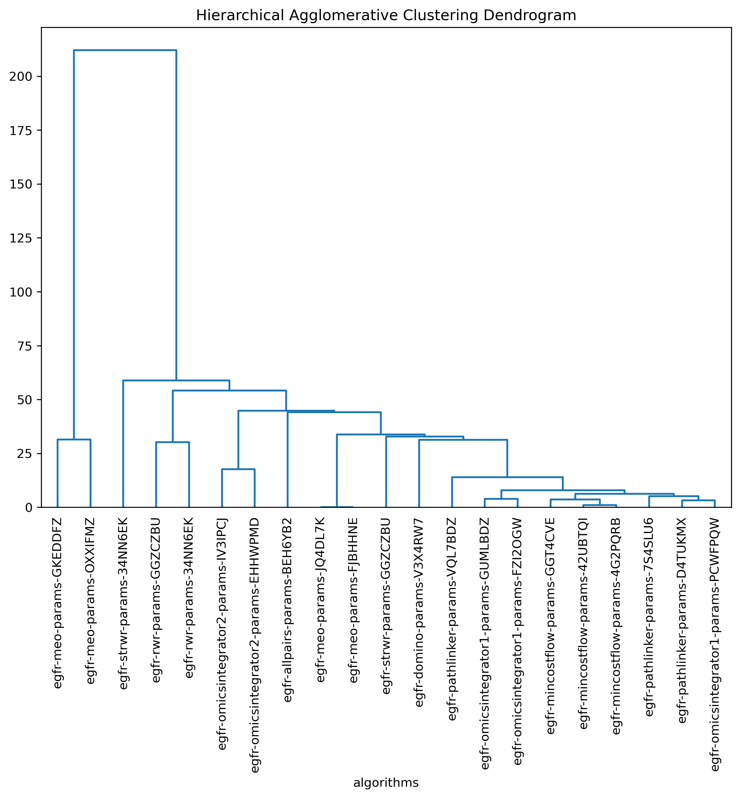
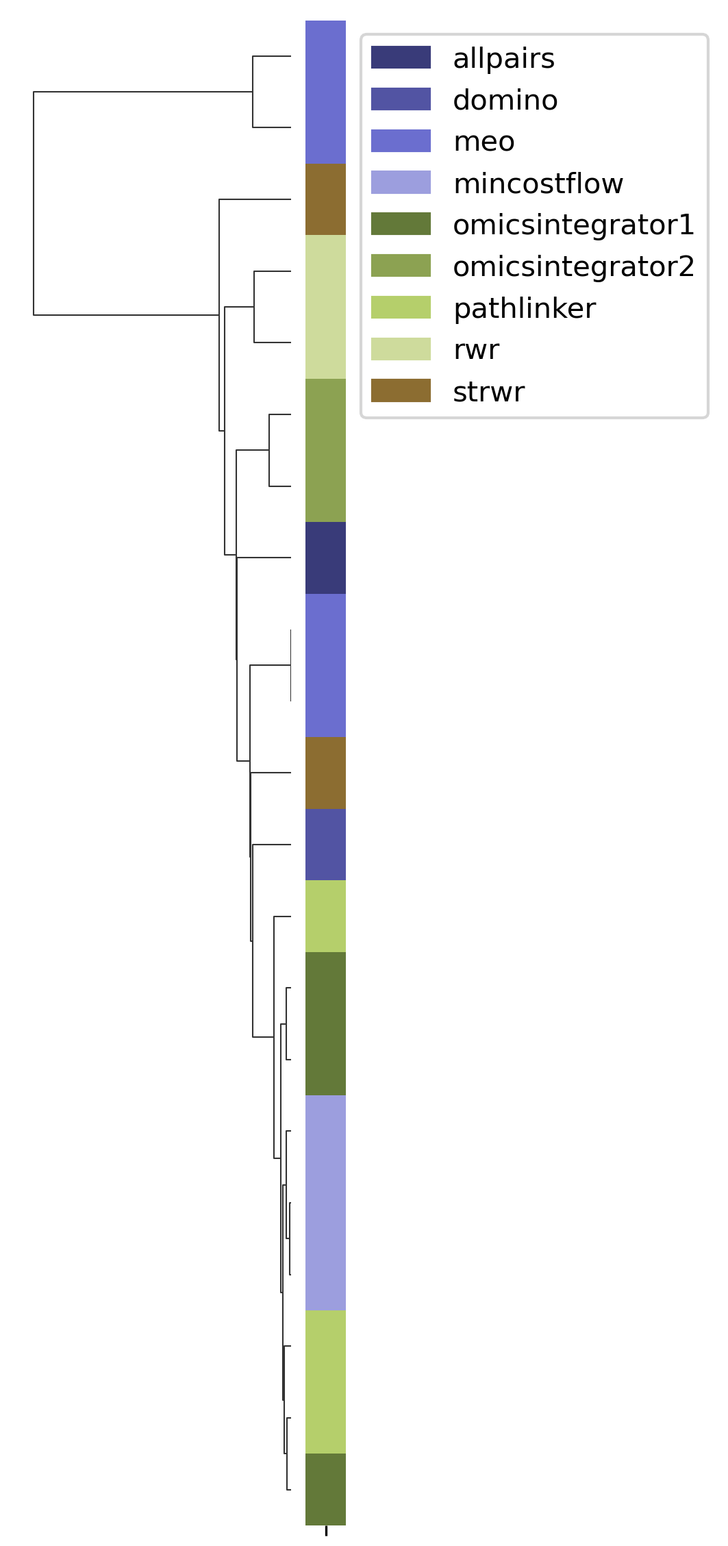
HAC visualizations help compare which algorithms and parameter settings produce similar pathway structures. Tight clusters indicate similar output behavior, while isolated branches may reveal unique results.

Principal component analysis

1. Open the PCA image

In your file explorer, go to output/intermediate/egfr-ml/pca.png and open it locally.

SPRAS also includes PCA to visualize variation across pathway outputs. Each point represents a pathway, placed based on its overall network structure. Pathways that cluster together in PCA space are more similar, while those farther apart differ in their reconstructed subnetworks.

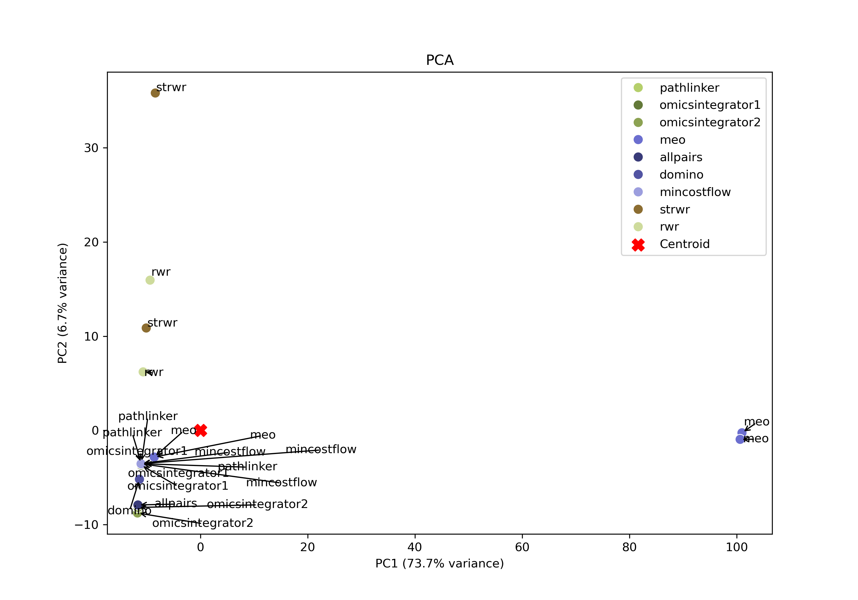
PCA may help identify patterns such as clusters of similar algorithms outputs, parameter sensitivities, and/or outlier outputs.

Jaccard similarity

1. Open the jaccard heatmap image

In your file explorer, go to output/intermediate/egfr-ml/jaccard-heatmap.png and open it locally.

SPRAS computes pairwise jaccard similarity between pathway outputs to measure how much overlap exists between their reconstructed subnetworks. The heatmap visualizes how similar the output pathways are between algorithms and their parameter settings.

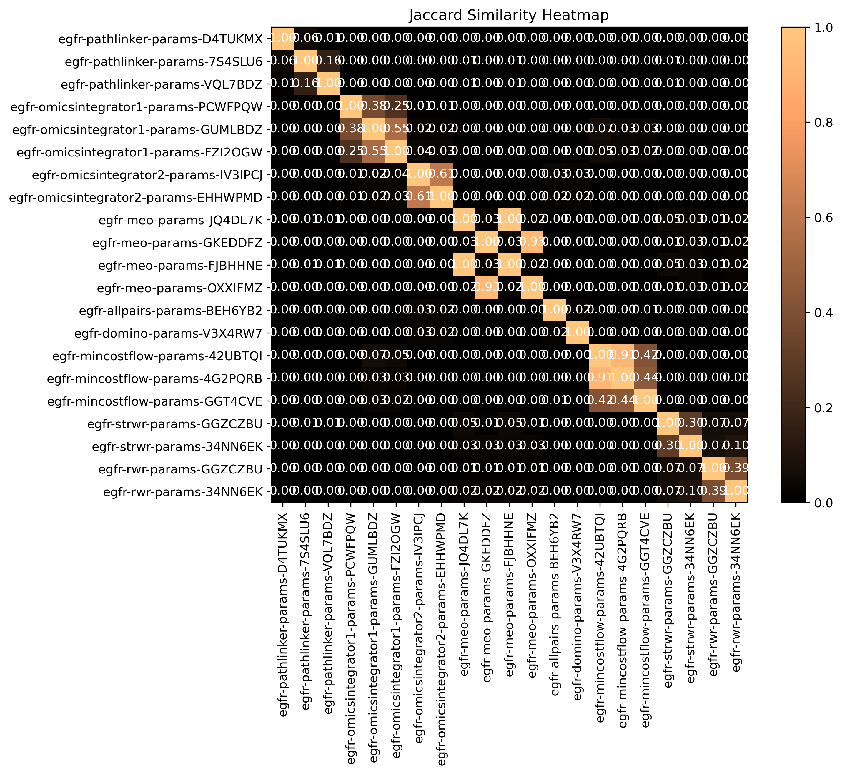
Higher similarity values indicate that pathways share many of the same edges, while lower values suggest distinct reconstructions.

References

[1]

Kanehisa, M., Furumichi, M., Sato, Y., Matsuura, Y. and Ishiguro-Watanabe, M.; KEGG: biological systems database as a model of the real world. Nucleic Acids Res. 53, D672-D677 (2025).

[2]

Kanehisa, M; Toward understanding the origin and evolution of cellular organisms. Protein Sci. 28, 1947-1951 (2019)

[3]

Kanehisa, M. and Goto, S.; KEGG: Kyoto Encyclopedia of Genes and Genomes. Nucleic Acids Res. 28, 27-30 (2000).

[4] (1,2)

Köksal AS, Beck K, Cronin DR, McKenna A, Camp AND, Srivastava S, MacGilvray ME, Bodík R, Wolf-Yadlin A, Fraenkel E, Fisher J, Gitter A. Synthesizing Signaling Pathways from Temporal Phosphoproteomic Data. Cell Rep. 2018 Sep 25;24(13):3607-3618. doi: 10.1016/j.celrep.2018.08.085. PMID: 30257219; PMCID: PMC6295338.